Configuration File¶

Functions¶

TTiP allows the creation of functions using either one of the built in function builders, or by writing expressions.

The simplest functions can be defined as:

<name>: <expression>

e.g.:

radial: 1/sqrt(x^2 + y^2)

Functions can also be interim functions. An interim function is one that is used as a component in other functions but is not used directly by the section. To define an interim function, start the function name with an ‘_’:

_<name>: <expression>

Interim functions can then be used by name:

_foo: 10 + x*y
bar: foo^2

TTiP also offers predefined function builders which offer some useful functionality. Function builders are used to create specific functions in the TTiP configuration file and are defined by setting the various properties with respect to a name, using the form:

<name>.<property>: <value>

Each function builder must define the type property, along with the relevent properties for the selected type. e.g.:

foo.type: gaussian
foo.mean: 0.5
foo.sd: 0.1
foo.scale: 10

Available function builders are:

Condition
Constant
File
Gaussian

Condition¶

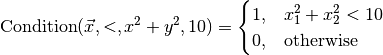
The condition function allows the user to create a stepped function using an operator alongside a left and right hand side (lhs and rhs respectively).

Args:

operator (str): The operator to use.
lhs (str): An expression for the left hand side.
rhs (str): An expression for the right hand side.

The exact formula is:

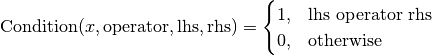
$\text{Condition}(x, \text{operator}, \text{lhs}, \text{rhs}) = \begin{cases} 1, &\text{lhs} \text{ operator } \text{rhs}\\ 0, &\text{otherwise} \end{cases}$

Where:

operator is an operator (‘<’, ‘>’, ‘<=’, ‘==’, …)
lhs is an expression for the left hand side
rhs is an expression for the right hand side

e.g.

$\text{Condition}(\vec{x}, <, x^2 + y^2, 10) = \begin{cases} 1, & x_1^2 + x_2^2 < 10\\ 0, &\text{otherwise} \end{cases}$

Constant¶

The Constant function creates a uniform function of value across the whole domain.

Args:

value (numerical): The constant value.

The exact formula is:

$\text{constant}(x, \text{value}) = \text{value}$

Where:

value is a scalar

File¶

The File function creates an function interpolated from data in a file.

Args:

path (str): The path to the file to interpolate.

The file must be a csv (optionally with a commented header row), where the first n columns represent the coords and the final column is the value at the coordinate.

e.g. For a 2D problem:

# x, y, val
0.0, 0.0, 10.0
0.1, 0.0, 9.0
0.2, 0.0, 8.0
0.3, 0.0, 7.0
...

Cubic interpolation is used for 1-D or 2-D problems, while linear interpolation is used for higher dimensional problems.

Gaussian¶

The Gaussian function creates a symmetric function with a peak equal to the scale at the location defined by mean. As the distance from this peak increases, the function decays exponentially. This decay is controlled by sd.

Args:

mean (numerical): The mean for the function.
sd (numerical): The standard deviation of the function.
scale (numerical): The amount to scale the function by.

The exact formula is:

$\text{gaussian}(x, \text{mean}, \text{sd}, \text{scale}) = \text{scale}\times e^{-\frac{1}{2}\left(\frac{x-\text{mean}}{\text{sd}}\right) \cdot\left(\frac{x-\text{mean}}{\text{sd}}\right)}$

Where:

mean is a vector (comma seperated list) of length dim(x), or a scalar value that will be broadcast to a vector.
sd is a vector (comma seperated list) of length dim(x), or a scalar value that will be broadcast to a vector.
scale is a scalar value

File Sections¶

Each section is defined properly in the example config:

[PHYSICS]
# The physics section is used to enable/disable physical limits.

# limit_conductivity (bool): Enable the lower limit on conductivity?
# limit_flux (bool): Enable flux limiting?
limit_conductivity: on
limit_flux: on

[SOLVER]
# The solver section defines which solver to use and where to store the
# results.

# file_path (string): The path to store the result in.
# method (string): The method to use for time dependant problems.
#     Avalilable options are: ForwardEuler, BackwardEuler, CrankNicolson, and Theta.
# theta (float): **Theta only** The theta parameter for a theta model solve.
file_path: ttip_results/result.pvd
method: CrankNicolson

[MESH]
# The mesh is defined by a type and parameters.
# Mesh types include all UtilityMeshes in firedrake as well as the option to
# read from a file.
#
# To create a mesh from file, stored at <filename>, use:
# type: Mesh
# params: <filename>
#
# For information on Utility meshes, see the firedrake docs:
# https://firedrakeproject.org/firedrake.html#module-firedrake.utility_meshes

# type (string): Which Mesh builder to use.
# params (comma seperated list): The params for the given mesh builder.
# element (string): The type of element to use in the mesh.
# order (int): The order of the element to use in the mesh.
type: Box
params: 20, 20, 20, 4e-5, 4e-5, 4e-5

element: CG
order: 1


[PARAMETERS]
# Any parameters are defined by name.
# For example the below defines the density parameter.
# A parameter will only be used if one of the mixins requests it.
# Parameters follow the same pattern as other functions which can be read about
# below.
#
# No defaults are provided. Options are given below:
# atomic_number
# coulomb_ln
# electron_density
# ion_density
# ionisation

[SOURCES]
# Any sources that are defined here will be summed to produce a final source
# term.
# Sources follow the same pattern as other functions which can be read about
# below.
#
# The default is no source term.
# default_source: 0

[BOUNDARIES]
# Boundary conditions can be defined for each boundary surface in the mesh.
# Problems can have no boundary conditions by leaving this section empty,
# otherwise each surface must have 1 boundary condition, to define a condition
# on all surfaces use 'all'.

# <name>.boundary_type (string): The type of boundary condition
#                                (dirichlet, neuman, robin)
# <name>.surface (comma separated list or 'all'): The surface the condition
#                                                 applies for.
# If using dirichlet, you should also define:
#     - g (the value on the boundary). This should be either a scalar value,
#       or a function defined as described at the bottom of this document.
#       e.g. bound.g.type: Constant ...
# If using neuman (not available yet!), you should also define:
#     - g (the derivative on the boundary). This should be a scalar or
#       function.
# If using robin (not available yet!), you should also define:
#     - alpha
#     - g
#fixed.boundary_type: dirichlet
#fixed.g: 100
#fixed.surface: 1, 2, 3, 4, 5, 6

[TIME]
# Time is used to define any time dependency in the problem.
# If this section is left blank, the problem is assumed to be steady state.
# Only 2 (any 2) of the settings in this section are needed, and the third can
# be calculated.

# steps (int): The number of steps to take.
# dt (float): The length of each time step.
# max_t (float): The maximum time to step until.
#steps: 10
#dt: 1e-12
#max_t: 1e-13

[INITIALVALUE]
# Initial values follow the same pattern as sources.
#
# Defaults to 0 across the mesh.
# default_initial_value: 0


# Functions:
# To define a function in TTiP, we use the following format
# <name>.type: <type>
# <name>.<param1>: <value1>
# ...
#
# For details on available functions and their parameters, please see the main
# documentation for TTiP.